Gallery: Multipatch wave equation
The Llama code is a 3-dimensional multiblock infrastructure for Cactus based on Carpet. It provides different patch systems that cover the simulation domain by a set of overlapping patches. Each of these patches has local cooordinates with a well-defined relation to global Cartesian coordinates. Information between the different patches is communicated via interpolation in the overlap zones.
Here we show an example evolution of a wave equation on a Kerr background using the "Thornburg2004nc" patch-system, consisting of 90 degree by 90 degree wedges centred on each of the +x, -x, +y, -y, +z, -z coordinate axes. This provides a complete covering of a region between rmin and rmax with smooth inner and outer boundaries. The initial data is an l=2, m=2 spherical harmonic in the angular directions, and a Gaussian in the radial direction. An alternative patch system, "Thornburg2004", adds a cubical patch enclosing r < rmin in which standard Carpet box-in-box mesh refinement can be employed. This is used in the GW150914 gravitational wave gallery example.
We ask that if you make use of the Llama code, then please cite Llama, the Einstein Toolkit, the Carpet mesh-refinement driver and Cactus.
Simulation details
Computational details
| Parameter File | Kerr-Schild_Multipole.par |
|---|---|
| Submission command | simfactory/bin/sim create-submit Kerr-Schild_Multipole --parfile arrangements/Llama/LlamaWaveToy/par/Kerr-Schild_Multipole.par |
| Total memory | 800 MB |
| Run time | A little over 1 minute using 56 MPI tasks and 56 cores on Frontera; or about 10 minutes on two laptop cores |
| Results (gzip 227MB, uncompressed 460MB) | Kerr-Schild_Multipole-20250522.tar.gz |
This example was last tested on May-22-2025.
Examples
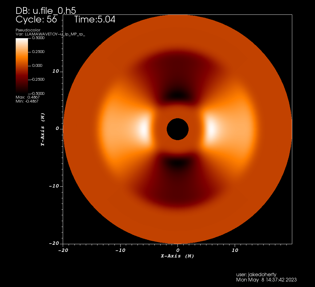
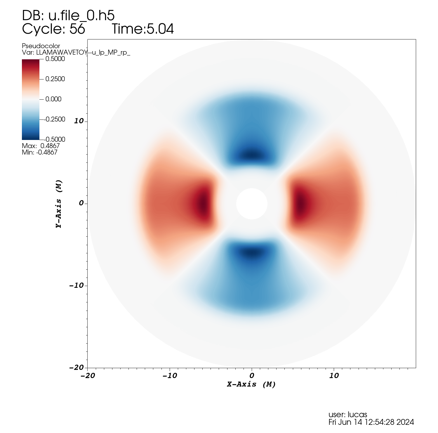
Projection into the xy plane of an l=2, m=2 multipole evolved with the wave equation on a spherical grid made of 6 coordinate patches. Images created using the VisIt file Kerr-Schild_Multipole.session and Python script plot.py.
Using the VisIt session file
- Get the VisIt session file.
- Run the
visitexecutable. - Navigate to
File > Restore session with sources .... - On the new window, select the visit session file downloaded in step 1.
- On the new window, making sure that
SOURCE00is selected in theSource Identifierspane, click on the...button of theSourcepane. - On the new window, navigate to the folder where the simulation's
HDF5files are located. - On the
Filespane, locate and click on theu.file_* databaseicon. - Click the
OKbutton. - Click the
OKbutton. - At this point, the plot should be displayed on the main plot window. Any warnings can be safely dismissed.
Creating the plots manually
If the file structure is different than expected in the saved *.session files above, the following VisIt directions might help:
- Run the
visitexecutable. - Click
Open - On the new window, in the
Directoriespanel, navigate to the location of the simulation'sHDF5output - On the
Filespanel, navigate to theu.file_* databaseentry and click it. The database will turn blue, indicating that it is selected. - On the
Open file as typedropdown menu, selectCarpetHDF5. Click theOKbutton. - On the main window, under the
Plotspanel, clickAdd > Pseudocolor > LLAMAWAVETOY--u_lp_MP_rp_. - On the main window, under the
Plotspanel, clickOperators > Slicing > Slice. - On the main window, under the
Plotspanel, open the dropdown menu of thePseudocolor - Slice(LLAMAWAVETOY--u_lp_MP_rp_) - Under the dropdown menu of
Pseudocolor - Slice(LLAMAWAVETOY--u_lp_MP_rp_), double-click theSlicecomponent. - On the new
Slice operator attributeswindow, under theNormalpanel, select theZ Axisradio button. Click apply. - Close the
Slice operator attributeswindow. - On the main window, under the
Plotspanel, clickDraw. - On the main window, under the dropdown menu of
Pseudocolor - Slice(LLAMAWAVETOY--u_lp_MP_rp_)double-click onPseudocolor. - On the new
Pseudocolor plot attributeswindow, on theData > Scale > Limitspanel, check theMinimumandMaximumcheckboxes. Change theMinimumfield to-0.5andMaximumfield to0.5. - On the same window, under the
Colorpanel, click theColor Tabledropdown menu and select theorangehotitem. Check theInvertcheckbox. - Click
Applyand close thePseudocolor plot attributeswindow. - On the visualization window (the one that contains the plot) click on the
Swap background and foreground colorsbutton, represented by a black triangle with two green arrows. - On the main window, under the
Timepanel, type56on the time field and press theENTERkey on your keyboard. The plot obtained reproduces exactly the first image on this gallery page. Users are encouraged to try and experiment with other settings, particularly other color maps and simulation times or 2D slices. - To save the figure, on the main window go to
File > Set save options .... - On the new window, under the
Filenamepanel, set theOutput directoryfield to the desired location. ClickApplyand close this window. - Click on
File > Save windowto save the image.
Using the Python script
The Python script needs to be executed within VisIt's Python parser. Download the script and navigate to the directory where the visit binary is located (this is not necessary if VisIt is in your PATH environment variable). In your command line, issue
visit -cli -nowin -s plot.py <HDF5 dir> <output dir> <output name>
where
<HDF5 dir>is the directory containing the outputHDF5files.<output dir>is the directory where the image will be saved.<output name>is the name of the output file (excluding the file extension).