![]()
CarpetX is a Cactus driver thorn based on AMReX, a software framework for block-structured AMR (adaptive mesh refinement). CarpetX is intended for the Einstein Toolkit.
Driver thorns are special modules that provide distributed data structures, refine meshes, perform memory allocation, and interfaces to parallel computing hardware and software. In short, they provide all the low-level basic infrastructure needed for any scientific simulation.
TODO: We should have some words explaining what CarpetX is.
There are a few standard images for CarpetX.
There are a set of them in the docker directory of CarpetX’s main GitHub repository. These build the various packages that CarpetX depends on mostly by hand. This is probably the more official set of images.
Another is build from this Dockerfile. This image is based on Spack, a flexible, python-based system for installing packages. This image contains optionlist files for Cactus in /usr/cactus/local-cpu.cfg and /usr/local-gpu.cfg. This image also contains two versions of the hpctoolkit tool, one that is cuda-enabled and one that is not. This rather beefy image is nearly 40GB in size, but it provides you with a complete set of tools for building and running CarpetX, Cactus, and the various development projects taking place within that framework. The image is maintained at docker.io/stevenrbrandt/etworkshop.
If you are running on a cluster with Singularity installed, you can compile the image as follows:
1singularity build -F /work/sbrandt/images/etworkshop.simg \
2    docker://stevenrbrandt/etworkshop
You can run the image using something like the following:
1srun singularity exec --nv \
2     --bind /var/spool --bind /work \
3     --bind /etc/ssh/ssh_known_hosts \
4     exec /work/sbrandt/images/etworkshop.simg cactus_sim my_parfile.par
Whether you choose to use one of the above images, or create an installation based on what you find in the dockerfiles for the above images, we wish you luck in your compiling and running efforts.
CCL files are used to define cactus thorns and customize its behavior. In this section, we shall discuss the additions that CarpetX brigs to these files, but we shall not teach users how to write them from scratch. In order to learn more, refer to Sec. C of the Cactus user guide provided in the doc folder of all distributions.
Users may need to require certain thorns explicitly in configuration.ccl files when using CarpetX APIs or schedule functions at specific bins provided by thorns in the CarpetX arrangement. These thorn-specific additions are documented in the thorn’s section of this text.
An important point to note is that CarpetX strongly enforces read, write and location statement correctness at runtime and compile time as declared in schedule.ccl files. This means that one is not able to write to a variable declared as READ. CarpetX also marks points in regions as valid or invalid and impedes user of reading from invalid data points. These extra measures help users prevent common memory and region access bugs.
In their C++ code, users should always use the DECLARE_CCTK_ARGUMENTSX_<scheduled function name> macro to ensure that only the objects declared in the function’s schedule block in schedule.ccl are brought into scope, as well as other objects necessary for working with CarpetX.
The centering of a grid function is declared via CENTERING=<centering-code>, where <centering-code> is a three-letter code containing any combination of either c or v, representing cell centering and vertex centering, respectively in interface.ccl files. For example, to declare a group of variables as being cell centered, one would use
1  CCTK_<type> <group-name> CENTERING={ccc}
2  {
3    ...
4  } "A group of variables"
Similarly, for a vertex centered group one would use
1  CCTK_<type> <group-name> CENTERING={vvv}
2  {
3    ...
4  } "A group of variables"
Note that it is possible to mix centering indexes. For example, to have a quantity centered at faces in the x direction, one would write
1  CCTK_<type> <group-name> CENTERING={cvv}
2  {
3    ...
4  } "A group of variables"
Not also that if no CENTERING is specified, CarpetX assumes that the variable group is vertex centered in all directions.
Finally, it is very important to match the centering description in interface files with the description passed to loop API template arguments. See Sec. 5 for details.
Tags are declared in interface statements (in interface.ccl) with the TAGS=<tags> syntax. The <tags> declaration consists of a single quote string (marked by ’) with space separated key-value pars of the form key="value". For example, a tagged interface declaration will be similar to the following
1  CCTK_<type> <group-name> TAGS=’key_1="key1" key_2="key2" ...’
2  {
3    ...
4  } "A group of variables"
We will now list the tags supported by CarpetX and describe their usage.
Marks a group of grid variables as the RHS (right-hand side) of a system. ODESolvers uses this information to perform time steps and update a state vector (See Sec. 6 for more information). For example, in
1  CCTK_<type> state_vector TAGS=’rhs="right_hand_side"’
2  {
3    ...
4  } "A group of variables representing the PDE system state"
5
6  CCTK_<type> right_hand_side
7  {
8    ...
9  } "A group of variables representing the PDE RHS"
the rhs="right_hand_side" tag indicates that the group named state_vector has a corresponding RHS group named right_hand_side.
1  CCTK_<type> state_vector TAGS=’rhs="right_hand_side"’
2  {
3    ...
4  } "A group of variables representing the PDE system state"
Indicates that the groups of variables contained on this tag must be marked as invalid if there are any changes to the group being declared. For example, in
1  CCTK_<type> parent_group TAGS=’dependents="child1 child2"’
2  {
3    ...
4  } "A group of real variables"
the tag dependents="child1 child2" indicates that parent_group has two dependent groups, child1 and child2. Whenever CarpetX writes to variables in parent_group, variables in child1 and child2 are marked as invalid and cannot be read from unless written to again.
Indicates that a variable group must be saved as a simulation checkpoint. Cactus and CarpetX can then later recover the saved checkpoint variables and restore the simulation state to continue evolution from there. Usually, only state vectors are checkpointed (See Chap. A3 of the Cactususer manual for further details). For example, in
1  CCTK_<type> state_vector TAGS=’checkpoint="yes"’
2  {
3    ...
4  } "A group of real variables describing the simulation state"
5
6  CCTK_<type> right_hand_side TAGS=’checkpoint="no"’
7  {
8    ...
9  } "A group of real variables describing the simulation RHS"
the simulation state, represented by the state_vector group is checkpointed, while the right_hand_side group is not.
The parameters CarpetX::checkpoint_method and CarpetX::recover_method control CarpetX’s behavior during variable checkpointing and recovery, respectively. Both parameters accept the same keyword values, described in Tab. 1
| Setting value | Effect |
| error | Abort with error instead of checkpointing/recovering (default) |
| openpmd | Uses openpmd formatted files for writing checkpoints |
| silo | Uses silo files for writing checkpoints |
TODO: Using TerminationTrigger to control checkpointing does not work yet.
To control when a checkpoint is to be produced, users first need to set the flash parameter Cactus::terminate, which controls under which conditions a simulation is to be terminated (see Sec. D5.2 of the Cactus user guide for further details on possible values for this parameter). After that, they can control various aspects of the checkpoint files produced, such as name and checkpoint file production on termination by setting parameters in the IO thorn. This is an infrastructure thorn that is always active and communicates its settings to CarpetX, which is effectively responsible for writing data to disk. To see all available parameters that can be set in IO, read the file Cactus/repos/cactusbase/IOUtil/param.ccl lines 137-205. These parameters are well documented in this file.
Additionally, it is imperative to set the flash’s presync mode to "presync-only" by adding Cactus::presync_mode = "presync-only" to the simulation’s parameter file. Failure to do so will cause the recovered checkpoints to be valid only on the interior and not on ghosts and boundaries (See Sec. D5.2 of the Cactus user guide for more information on presync modes).
As an example, we present an excerpt of a parameter file for a simulation that ends after simulation time reaches \(t=100\), but we allow Cactus running for only 1 minute of wall time. For the physical system being simulated, such execution time is not enough for the system to reach \(t=100\), thus the execution of Cactus will be terminated before the system is completely evolved. We would like to be able to recover from the last iteration performed by the system in subsequent executions of Cactus. To do that, we will configure the IO thorn to produce checkpoint files upon Cactus termination.
1  # Required in order to recover successfully
2  Cactus::presync_mode = "presync-only"
3
4  # The type of checkpoint and recovery files that should be used
5  CarpetX::checkpoint_method = "openpmd"
6  CarpetX::recover_method    = "openpmd"
7
8  # Schedule termination of the simulation for 1 minute of wall time
9  Cactus::terminate       = "runtime"
10  Cactus::cctk_final_time = 100.0
11  Cactus::max_runtime     = 1.0
12
13  # Configure IO to produce checkpoint files before terminating
14  IO::checkpoint_ID           = no
15  IO::recover                 = "autoprobe"
16  IO::out_proc_every          = 2
17  IO::checkpoint_on_terminate = yes
18  IO::checkpoint_dir          = "../checkpoints"
19  IO::recover_dir             = "../checkpoints"
20  IO::abort_on_io_errors      = yes
The parity tag controls a tensor’s reflection symmetries about the x, y and z axes. There are 3 parities for each tensor component, representing the symmetries about the 3 spatial axes.
For example, a scalar, has parities={+1 +1 +1}, which indicates that no sign changes take place when the quantity is reflected around the axes. If no parities tag is present in a variable group declaration, it is assumed to be a scalar and parities={+1 +1 +1} is implicitly assumed. For a vector, the parities={-1 +1 +1 +1 -1 +1 +1 +1 -1} tag indicates in the first triad of numbers that the vector’s x component changes sign while being reflected in the x direction, the second triad indicates that the y component changes sign while reflected in the y direction and the third triad indicates that the z component changes sign while being reflected in the z direction. As an example, let us look at the parities of the energy momentum tensor in general relativity as declared in the interface.ccl file of the TmunuBaseX thorn included in CarpetX :
1# The T_{tt} component represents the energy density and
2# is stored as a scalar. The parities={+1 +1 +1} tag is implicit.
3CCTK_REAL eTtt TAGS=’checkpoint="no"’ TYPE=gf "T_00"
4
5# The T_{ti} components of the tensor are a vector of three entries.
6# Each component changes sign when reflected on their respective axes.
7CCTK_REAL eTti TAGS=’parities={-1 +1 +1    +1 -1 +1    +1 +1 -1} checkpoint="no"’ TYPE=gf
8{
9    eTtx eTty eTtz
10} "T_0i"
11
12# The T_{ij} components form a rank 2 tensor of 3 spatial dimensions.
13# Each index triplet represents a component in the tensor.
14CCTK_REAL eTij TAGS=’parities={+1 +1 +1    -1 -1 +1    -1 +1 -1    +1 +1 +1    +1 -1 -1    +1 +1 +1} checkpoint="no"’ TYPE=gf
15{
16    eTxx eTxy eTxz eTyy eTyz eTzz
17} "T_ij"
18
19# The parities tag on this tensor indicates that:
20# * The xx component does not change sign.
21# * The xy component changes sign while reflecting on either x or y.
22# * The xz component changes sign while reflecting on either x or z.
23# * The yy component does not change sign.
24# * The yz component changes sign while reflecting on either y or z.
25# * The zz component does not change sign.
In this section, we will describe CarpetX’s parameters used for describing the simulation domain. Currently, CarpetX supports only Cartesian grids. To control the grid’s extents, users must utilize parameters described in Tab. 2. To control the number of cells in each direction, users must set the parameters described in Tab. 3. Finally, to control the number of ghost zones in the grid, users must set the parameters described in Tab. 4. It is important to note that the size of all ghost zones can be set at once via ghost_size parameter or via the ghost_size_xyz family of parameters if ghost_size is set to \(-1\)
| Parameter | Description | Default value |
| xmin | Minimum value of the grid in the \(x\) direction | \(-1.0\) |
| xmax | Maximum value of the grid in the \(x\) direction | \(1.0\) |
| ymin | Minimum value of the grid in the \(y\) direction | \(-1.0\) |
| ymax | Maximum value of the grid in the \(y\) direction | \(1.0\) |
| zmin | Minimum value of the grid in the \(z\) direction | \(-1.0\) |
| zmax | Maximum value of the grid in the \(z\) direction | \(1.0\) |
| Parameter | Description | Default value |
| ncells_x | Number of grid cells in the \(x\) direction | \(128\) |
| ncells_y | Number of grid cells in the \(y\) direction | \(128\) |
| ncells_z | Number of grid cells in the \(z\) direction | \(128\) |
| Parameter | Description | Default value |
| ghost_size | Number of grid cells in all directions. | \(-1\) |
| ghost_size_x | Number of ghost zones in the \(x\) direction | \(1\) |
| ghost_size_y | Number of ghost zones in the \(y\) direction | \(1\) |
| ghost_size_z | Number of ghost zones in the \(z\) direction | \(1\) |
In CarpetX loops over grid elements are not written explicitly. Operations that are to be executed for every grid element (cells, edges or points) are specified via C++ lambda functions, also known as closures or anonymous functions.
These objects behave like regular C++ functions, but can be defined inline, that is, on the body of a function or as an argument to another function.
An important concept to grasp with lambda function is captures. If a lambda (let us call this the child function) is defined in the body of an outer function (let us call this the parent function), the child can access variables defined in the parent function, provided that these variables are captured. The two most relevant modes of capture while using CarpetX are capture by reference (denoted with the & sign in the square brackets denoting the start of the lambda) and capture by value (denoted by an = sign inside the square brackets of the lambda declaration).
When running on GPUs, captures by value are required and captures by reference are forbidden. This is because data must be copied from host (CPU side) memory to device (GPU side) memory in order to be executed.
The API for writing loops in CarpetX is provided by the Loop thorn. To use it, one must add
1 REQUIRES Loop
to the thorn’s configuration.ccl file and
1    INHERITS: CarpetXRegrid
2    USES INCLUDE HEADER: loop_device.hxx
to the thorn’s interface.ccl file. Furthermore, one must include the Loop API header file in all source files where the API is needed by adding
1 #include <loop_device.hxx>
to the beginning of the source file.
Before actually writing any code that iterates over grid elements, one must choose which elements are to be iterated over. We shall refer to the set of points in the grid hierarchy that will be iterated over when a loop is executed as a Loop region. The following regions are defined in the Loop API:
All: This region refers to all points contained in the grid. Denoted in code by the all suffix.
Interior: This region refers to the interior of the grid. Denoted in code by the int prefix.
Outermost interior: This region refers to the outermost ”boundary” points in the interior. They correspond to points that are shifted inwards by = cctk_nghostzones[3] from those that CarpetX identifies as boundary points. From the perspective of CarpetX (or AMReX), these do not belong in the outer boundary, but rather the interior. This excludes ghost faces, but includes ghost edges/corners on non-ghost faces. Loop over faces first, then edges, then corners. Denoted in code by the outermost_int suffix.
TODO: Picture of grid regions
Loop API functions are methods of the GridDescBaseDevice class which contain functions for looping over grid elements on the CPU or GPU, respectively. The macro DECLARE_CCTK_ARGUMENTSX_FUNCTION_NAME provides a variable called grid, which is an instance of either of these classes. The name of each looping method is formed according to
loop_ + <loop region>+ [_device]
For example, to loop over boundaries using the CPU one would call
1 grid.loop_bnd<...>(...);
To obtain a GPU equivalent version, one would simply append _device to the function name. Thus, for example, to loop over the interior using a GPU, one would call
1 grid.loop_int_device<...>(...);
Let us now look at the required parameter of loop methods. The typical signature is as follows
1  template <int CI, int CJ, int CK, ..., typename F>
2  void loop_REG_PU(const vect<int, dim> &group_nghostzones, const F &f);
The template parameters meanings are as follows:
CI: Centering index for the first grid direction. Must be set explicitly and be either 0 or 1. 0 means that this direction will be looped over grid vertices, while 1 means that it will be looped over cell centers.
CJ: Centering index for the second grid direction. Must be set explicitly and be either 0 or 1. 0 means that this direction will be looped over grid vertices, while 1 means that it will be looped over cell centers.
CK: Centering index for the third grid direction. Must be set explicitly and be either 0 or 1. 0 means that this direction will be looped over grid vertices, while 1 means that it will be looped over cell centers.
F: The type signature of the lambda function passed to the loop. It is not required to be set explicitly and is automatically deduced by the compiler.
Note that centering indexes can be mixed: setting the indices to \((1,0,0)\), for instance, creates loops over faces on the x direction. Function parameter meanings are as follows:
group_nghostzones: The number of ghost zones in each direction of the grid. This can be obtained by calling grid.nghostzones.
f: The C++ lambda to be executed on each step of the loop.
We shall now discuss the syntax and the available elements of the lambda functions that are to be fed to the Loop methods described in Section 5.2.
To start, let us be reminded of the general syntax of a lambda function in C++:
1  // append ; if assigning to a variable
2  [capture_parameter] (argument_list) -> return_type { function_body }
When running on GPUs, the capture_parameter field used should always be =, indicating pass by value (copy) rather than &, indicating pass by reference. The argument_list of the lambda should receive only one element of type PointDesc (which will be described on Sec. 5.4) and the lambda must return no value, which means that return_type can be omitted altogether.
This means that a typical lambda passed to a loop method will have the form
1  [=] (const Loop::PointDesc &p) {
2    // loop body
3  }
In addition, users can specify inlining (a compile-time optimization where the function call is replaced by its body) by using the CCTK_ATTRIBUTE_ALWAYS_INLINE macro and designate host or device availability via the CCTK_HOST or CCTK_DEVICE macros, respectively. These annotations are optional unless the compiler is unable to build a function due to an inability to automatically determine that it needs to be available for device usage, for example. However, when these annotations are desired, they must be placed in specific locations.
To mark a lambda for host usage, one would use:
1  [=] CCTK_HOST(const Loop::PointDesc &p) CCTK_ATTRIBUTE_ALWAYS_INLINE {
2    // loop body
3  }
For device usage, one would use:
1  [=] CCTK_DEVICE(const Loop::PointDesc &p) CCTK_ATTRIBUTE_ALWAYS_INLINE {
2    // loop body
3  }
For both host and device usage, one would use:
1  [=] CCTK_HOST CCTK_DEVICE(const Loop::PointDesc &p) CCTK_ATTRIBUTE_ALWAYS_INLINE {
2    // loop body
3  }
The PointDesc type provides a complete description of the current grid element in the loop. The following members are the ones that are expected to be used more often:
I: A 3-element array containing the grid point indices.
DI: A 3-element array containing the direction unit vectors from the current grind point.
X: A 3-element array containing the point’s coordinates.
DX: A 3-element array containing the point’s grid spacing.
iter: The current loop iteration.
BI: A 3-element array containing the outward boundary normal if the current point is the outermost interior point or zero otherwise.
In the body of a loop lambda, grid functions declared in the thorn’s interface.ccl file are available as GF3D2 objects, which are C++ wrappers around native Cactus grid functions. These objects are accessible by directly calling them as functions taking arrays of grid indices as input. Such indices, in turn can be obtained by directly accessing PointDesc members.
Let us now combine the elements describe thus far into a single example. Let us suppose that the following system of PDEs is implemented in Cactus:
\begin {align} \partial _t u & = \rho \label {eq:toy_loop_0}\\ \partial _t \rho & = \partial _x^2 u + \partial _y^2 u + \partial _z^2 u \label {eq:toy_loop_1} \end {align}
Let us suppose that the grid functions u and rho where made available, while grid functions u_rhs and rho_rhs are their corresponding RHS storage variables. The function that computes the RHS of Eqs. (??)-(??) can be written as
1extern "C" void LoopExample_RHS(CCTK_ARGUMENTS) {
2  DECLARE_CCTK_ARGUMENTS_LoopExample_RHS;
3  DECLARE_CCTK_PARAMETERS;
4
5  // The grid variable is implicitly defined via the CCTK macros
6  // A 0/1 in template parameters indicate that a grid is vertex/cell centered
7  grid.loop_int<0, 0, 0>(
8    grid.nghostzones,
9
10    // The loop lambda
11    [=] (const Loop::PointDesc &p) {
12      using std::pow;
13
14      const CCTK_REAL hx = p.DX[0] * p.dX[0];
15      const CCTK_REAL hy = p.DX[1] * p.dX[1];
16      const CCTK_REAL hz = p.DX[2] * p.dX[2];
17
18      const CCTK_REAL dudx = u(p.I - p.DI[0]) - 2 * u(p.I)
19        + u(p.I + p.DI[0])/hx;
20
21      const CCTK_REAL dudy = u(p.I - p.DI[1]) - 2 * u(p.I)
22        + u(p.I + p.DI[1])/hy;
23
24      const CCTK_REAL dudz = u(p.I - p.DI[2]) - 2 * u(p.I)
25        + u(p.I + p.DI[2])/hz;
26
27      u_rhs(p.I) = rho(p.I);
28      rho_rhs(p.I) = ddu;
29
30    } // Ending of the loop lambda
31  ); // Ending of the loop_int call
32}
If the user’s CPU supports SIMD instructions (see here for details), CarpetX is capable of vectorizing loops via the Arith thorn. To use it, users must add
1  USES INCLUDE HEADER: simd.hxx
2  USES INCLUDE HEADER: vect.hxx
to the top of their interface.ccl files, in addition to the other required headers.
While writing SIMD vectorized code, one has to keep in mind that grid functions are not a collection of CCTK_REAL values but a collection of Arith::simd<CCTK_REAL> real values, which is itself a collection of CCTK_REAL values. This becomes apparent when reading and writing to grid functions at a particular grid point. To see how these differences come about, let us study an example of initializing grid data using the SIMD API
1  extern "C" void SIMDExample_Initial(CCTK_ARGUMENTS) {
2  DECLARE_CCTK_ARGUMENTSX_SIMDExample_Initial;
3  DECLARE_CCTK_PARAMETERS;
4
5  using real = CCTK_REAL;
6  using vreal = Arith::simd<real>;
7
8  // This is the compile time determined vector size supported by the underlying CPU architecture
9  constexpr std::size_t vsize = std::tuple_size_v<vreal>;
10
11  // After passing the centering indices, size of the SIMD vectors is passed as template arguments
12  grid.loop_int_device<0, 0, 0, vsize>(
13    grid.nghostzones,
14
15    [=] (const Loop::PointDesc &p) {
16      // p.x is a scalar, but must be turned into a vector
17      const vreal x0 = p.x + Arith::iota<vreal>() * p.dx;
18      const real y0 = p.y;
19      const real z0 = p.z;
20
21      // The initialization function takes its inputs as vectors
22      vreal u0, rho0;
23      initial_data(x0, y0, z0, u0, rho0);
24
25      u.store(p.mask, p.I, u0);
26      rho.store(p.mask, p.I, rho0);
27    }
28  );
29}
In lines 5 and 6, we define aliases for the real scalar type CCTK_REAL and its associated vector type Arith::simd<real>. Values assigned to grid functions need to be of this type. In line 9, the vsize variable stores the size of the SIMD vectors of the target CPU. The constexpr keyword ensures that this expression is evaluated at compile time. In line 12, we call a loop API function with the three centering indices, discussed in Sec. 5.2, plus the extra vreal parameter which informs the loop method call that the loops will be vectorized.
At this point, it is very important to realize that loops can only be vectorized along the x direction. This is so because in SIMD vectors, entries must be sequential and internally, CarpetXstores 3D grid data as a flattened array and only the x direction is contiguous. Line 17 is responsible for the vectorization of the x direction. The Arith::iota<vreal>() instruction produces an array of contiguously increasing elements from 0 to vsize (not end inclusive) which then gets multiplied by p.dx and incremented by p.dx. As an illustrative example, let us suppose that \(\texttt {vsize} = 4\). In this case, \begin {equation} \texttt {Arith::iota<vreal>()} = \begin {pmatrix} 0\\ 1\\ 2\\ 3 \end {pmatrix} . \end {equation} The operation on line 17 becomes then \begin {equation} \texttt {x0} = \texttt {p.x} + \begin {pmatrix} 0\\ 1\\ 2\\ 3\\ \end {pmatrix} \texttt {p.dx} = \begin {pmatrix} \texttt {p.x}\\ \texttt {p.x} + \texttt {p.dx}\\ \texttt {p.x} + 2 * \texttt {p.dx}\\ \texttt {p.x} + 3 * \texttt {p.dx}\\ \end {pmatrix} \end {equation}
On lines 22 and 23, the initial_data function gets called and uses the vectorized x0 coordinates and scalar coordinates y0 and z0 to fill the vectorized initial data variables u0 and rho0 which then finally get assigned to their respective grid functions via the assign member on lines 25 and 26. The initial_data is arbitrary and user defined, but note that Arith overloads arithmetic operators and trigonometric functions, so it is straightforward to write code that uses vectorized and scalar variables together.
Let us now look at an example of writing derivatives and RHS functions with SIMD loops.
1  extern "C" void SIMDExample_RHS(CCTK_ARGUMENTS) {
2  DECLARE_CCTK_ARGUMENTSX_SIMDExample_RHS;
3  DECLARE_CCTK_PARAMETERS;
4
5  using vreal = Arith::simd<CCTK_REAL>;
6  constexpr std::size_t vsize = std::tuple_size_v<vreal>;
7
8  grid.loop_int_device<0, 0, 0, vsize>(
9    grid.nghostzones,
10
11    [=] (const Loop::PointDesc &p) {
12      using Arith::pow2;
13
14      const auto d2udx2 = (u(p.mask, p.I - p.DI[0]) - 2 * u(p.mask, p.I) + u(p.mask, p.I + p.DI[0]) ) / pow2(p.DX[0]);
15
16      const auto d2udy2 = (u(p.mask, p.I - p.DI[1]) - 2 * u(p.mask, p.I) + u(p.mask, p.I + p.DI[1]) ) / pow2(p.DX[1]);
17
18      const auto d2udz2 = (u(p.mask, p.I - p.DI[2]) - 2 * u(p.mask, p.I) + u(p.mask, p.I + p.DI[2]) ) / pow2(p.DX[2]);
19
20      const auto udot = rho(p.mask, p.I);
21      const auto rhodot = ddu;
22
23      u_rhs.store(p.mask, p.I, udot);
24      rho_rhs.store(p.mask, p.I, rhodot);
25    });
26  }
As previously mentioned, Arith overloads arithmetic operators, which makes writing mathematical expressions in vectorized loops no different from their non-vectorized counterparts. This is exemplified in lines 14-18 where second derivatives are being taken via finite differences approximations. Note once again in line 8 the presence of an extra template argument indicating the CPU’s vector sizes, the extra p.mask argument being passed on all invocations of grid functions and the use of the store method to assign computed values to the RHS grid functions.
TODO: Document fused SIMD operations
In CarpetX, time integration of PDEs via the Method of Lines is provided by the ODESolvers thorn. This makes time integration tightly coupled with the grid driver, allowing for more optimization opportunities and better integration.
From the user’s perspective, ODESolvers is very similar (and sometimes even more straightforward) the MoL thorn, but a few key differences need to be observed. Firstly, not all integrators available to MoL are available to ODESolvers. The list of all supported methods is displayed in Tab. 5. Method selection occurs via configuration file, by setting
1 ODESolvers::method = "Method name"
and the default method used if none other is set is ”RK2”.
| Name | Description |
| constant | The state vector is kept constant in time |
| Euler | Forward Euler method |
| RK2 | Explicit midpoint rule |
| RK3 | Runge-Kutta’s third-order method |
| RK4 | Classic RK4 method |
| SSPRK3 | Third-order Strong Stability Preserving Runge-Kutta |
| RKF78 | Runge-Kutta-Fehlberg 7(8) |
| DP87 | Dormand & Prince 8(7) |
| Implicit Euler | Implicit Euler method |
Additionally, users can set verbose output from the time integrator by setting
1 ODESolvers::verbose = "yes"
By default, this option is set to "no". Finally, to control the step size of the time integrator, it is possible to set the configuration parameter CarpetX::dtfac, which defaults to \(0.5\), is defined as \begin {equation} \texttt {dtfac} = \texttt {dt}/\min (\texttt {delta\_space}) \end {equation} where \(\min (\texttt {delta\_space})\) refers to the smallest step size defined in the CarpetX grid and dt is the time integrator step.
To actually perform time evolution, the PDE system of interest needs to be declared to Cactus as a set of Left-Hand Side (or LHS, or more commonly state vector) grid functions plus a set of Right-Hand Side (RHS) grid functions. The RHS grid functions correspond exactly to the right-hand side of the evolution equations while the state vectors stores the variables being derived in time in the current time step. More time steps can be stored internally, depending on the time integrator of choice, but this is an implementation detail that is supervised automatically by ODESolvers. To make this clear, consider the PDE system comprised of Eqs. (??)-(??). In this example, the state vector would be the set \((u,\rho )\) while the right-hand side would be all elements to the right of the equal signs. Note that derivative appearing on the RHS are only derivatives in space. By discretizing space with a grid and replacing continuous derivatives with finite approximations (by using finite differences, for instance) the time-space dependent PDE system now becomes a ODE system in time, with the state vector being the sought variables. By providing the RHS of the PDE system, ODESolvers can apply the configured time stepping method and compute the next time steps of the state vector.
To see how ODESolvers is used in practice, let us turn once again to the WaveToyX example, bundled with CarpetX. To begin, let us look at an excerpt from this example’s interface.ccl file
1  CCTK_REAL state TYPE=gf TAGS=’rhs="rhs" dependents="energy error"’
2  {
3    u
4    rho
5  } "Scalar wave state vector"
6
7  CCTK_REAL rhs TYPE=gf TAGS=’checkpoint="no"’
8  {
9    u_rhs
10    rho_rhs
11  } "RHS of scalar wave state vector"
12
13  ...
In lines 1-5, the group of real grid functions called state, consisting of grid function u and rho, is declared. The TYPE=gf entry indicates that the variables in this group are grid functions and the TAGS entry is particularly important in this instance, thus it is highly recommended that readers visit Sec. 3 for more information. The rhs="rhs" tag indicates that these grid functions have an associated RHS group, that is, a group of variables with grid functions responsible for storing the PDE system’s RHS and this group is called "rhs" which is defined later in lines 7-11. This information is used by ODESolvers while taking a time step and is tightly coupled to Cactus file parsers. In lines 7-11, the rhs group is declared with two real grid functions, u_rhs and rho_rhs. These variables will be responsible for holding the RHS data of the PDE, which will in turn be used by ODESolvers.
The next step is to schedule the execution of functions into their correct schedule groups. The most relevant schedule groups provided by ODESolvers are ODESolvers_RHS and ODESolvers_PostStep. The former is the group where one evaluates the RHS of the state vector everywhere on the grid and the latter is where boundary conditions are applied to the state vector, and projections are applied if necessary. For example, looking at WaveToyX’s schedule.ccl file, one sees
1  SCHEDULE WaveToyX_RHS IN ODESolvers_RHS
2  {
3    LANG: C
4    READS: state(everywhere)
5    WRITES: rhs(interior)
6    SYNC: rhs
7  } "Calculate scalar wave RHS"
8
9SCHEDULE WaveToyX_Energy IN ODESolvers_PostStep
10  {
11    LANG: C
12    READS: state(everywhere)
13    WRITES: energy(interior)
14    SYNC: energy
15  } "Calculate scalar wave energy density"
The schedule statement from lines 1-7 schedules the function that computes the RHS of the wave equation. Note that the function reads the state on the whole grid and writes to the RHS grid variables in the interior. With CarpetX, grid functions read and write statements are enforced: You cannot write to a variable which was declared as read only in the schedule.ccl file. Lines 9-15 exemplify the scheduling of a function in the ODESolvers_PostStep group, which is executed after ODESolvers_RHS during the time stepping loop. In this particular example, the scheduled function is computing the energy associated with the scalar wave equation system. These are all the required steps for using ODESolvers to solve a PDE system via the method of lines.
CarpetX supports fixed mesh refinement via the so called box-in-box paradigm. This capability is provided by the BoxInBox thorn. Using it is very simple and similar to Carpet’s CarpetRegrid2 usage.
| Name | Type | Possible Values | Default Value | Description |
| shape_n | String | "sphere" or "cube" | "sphere" | Shape of refined region |
| active_n | Boolean | "yes" or "no" | "yes" | Is this box active? |
| num_levels_n | Single integer | \([1,30]\) | \(1\) | Number of refinement levels for this box |
| position_x_n | Single real number | Any real | \(0.0\) | x-position of this box |
| position_y_n | Single real number | Any real | \(0.0\) | y-position of this box |
| position_z_n | Single real number | Any real | \(0.0\) | z-position of this box |
| radius_n | 30 element array of reals | \(-1.0\) or positive real | \(-1.0\) (radius ignored) | Radius of refined region for this level |
| radius_x_n | 30 element array of reals | \(-1.0\) or positive real | \(-1.0\) (radius ignored) | x-radius of refined region for this level |
| radius_y_n | 30 element array of reals | \(-1.0\) or positive real | \(-1.0\) (radius ignored) | y-radius of refined region for this level |
| radius_z_n | 30 element array of reals | \(-1.0\) or positive real | \(-1.0\) (radius ignored) | z-radius of refined region for this level |
All configuration of boxes and levels are performed within configuration files. BoxInBox supports adding 3 “boxes” or “centers”. Each box can be configured as summarized in Tab. 6. The n suffix should be replaced by 1, 2 or 3 for configuring the corresponding boxes. Each box can be shaped differently as either Cartesian-like cubes or spheres and support configuring up to 30 levels. Level’s positions and radii can be set independently for each dimension. Note that for each box the active, num_levels and position_(xyz) field are stored as grid scalars. Each of the 30 refinement level radii and x, y, z individual radii for each box are also stored as grid arrays. This allows these parameters to be changed during a simulation run, allowing for moving boxes. This is useful, for example, when implementing a puncture tracker.
These configurations are subjected to (and restricted by) two additional CarpetX configurations, namely CarpetX::regrid_every, which controls how many iterations should pass before checking if the box grid variables have changed and CarpetX::max_num_levels which controls the maximum number of allowed refinement levels.
As an example, we present a configuration file excerpt for creating two refinement boxes with the BoxInBox thorn
1  BoxInBox::num_regions = 2
2
3  BoxInBox::num_levels_1 = 2
4  BoxInBox::position_x_1 = -0.5
5  BoxInBox::radius_x_1[1] = 0.25
6  BoxInBox::radius_y_1[1] = 0.25
7  BoxInBox::radius_z_1[1] = 0.25
8
9  BoxInBox::num_levels_2 = 2
10  BoxInBox::position_x_2 = +0.5
11  BoxInBox::radius_x_2[1] = 0.25
12  BoxInBox::radius_y_2[1] = 0.25
13  BoxInBox::radius_z_2[1] = 0.25
Let us now suppose that one wishes to make the boxes set up in the above parameter file to move in a circle around the origin. This is not very useful in practice, but it illustrates important concepts that can be later applied to more complex tools, such as puncture trackers. The MovingBoxToy thorn bundled in CarpetX provides an example of how to achieve this. We shall now examine this implementation closely. Let us start by the examining the thorn’s interface.ccl file:
1  # Interface definition for thorn MovingBoxToy
2
3  IMPLEMENTS: MovingBoxToy
4
5  INHERITS: BoxInBox
The INHERITS statement in line 5 states that this thorn will write to grid functions provided in BoxInBox which control the refinement boxes parameters. Next, in the thorn’s param.ccl file we have
1  # Parameter definitions for thorn MovingBoxToy
2
3  shares: BoxInBox
4  USES CCTK_REAL position_x_1
5  USES CCTK_REAL position_x_2
Lines 3-5 declare that MovingBoxToy uses parameters position_x_1 and position_x_2 from BoxInBox. These declarations are required in order to access the initial positions of the boxes. Note that similar statements would be used if other parameters from BoxInBox were required.
Finally, in the schedule.ccl file we schedule the routine that will actually update the box positions, called MovingBoxToy_MoveBoxes:
1  # Schedule definitions for thorn MovingBoxToy
2
3  SCHEDULE MovingBoxToy_MoveBoxes AT postinitial BEFORE EstimateError
4  {
5    LANG: C
6    READS: BoxInBox::positions
7    WRITES: BoxInBox::positions
8  } "Update box positions"
9
10  SCHEDULE MovingBoxToy_MoveBoxes AT poststep BEFORE EstimateError
11  {
12    LANG: C
13    READS: BoxInBox::positions
14    WRITES: BoxInBox::positions
15  } "Update box positions"
Note that the routine is scheduled with AT poststep BEFORE EstimateError. This is important, since it is in the EstimateError bin that CarpetX’s AMR error grid function (see Sec. 7.2) will be updated thus any changes to box data should be scheduled before that.
Finally, the C++ routine MovingBoxToy_MoveBoxes that will actually update the boxes positions reads
1  extern "C" void MovingBoxToy_MoveBoxes(CCTK_ARGUMENTS) {
2    DECLARE_CCTK_ARGUMENTSX_MovingBoxToy_MoveBoxes;
3    DECLARE_CCTK_PARAMETERS;
4
5    using std::cos;
6
7    const CCTK_REAL omega{M_PI/4};
8
9    // Initial positions of box 1
10    const auto x0_1{position_x_1};
11
12    // Initial positions of box 2
13    const auto x0_2{position_x_2};
14
15    // Trajectory of box 1
16    position_x[0] = x0_1 * cos(omega * cctk_time);
17    position_y[0] = x0_1 * sin(omega * cctk_time);
18
19    // Trajectory of box 2
20    position_x[1] = x0_2 * cos(omega * cctk_time);
21    position_y[1] = x0_2 * sin(omega * cctk_time);
22  }
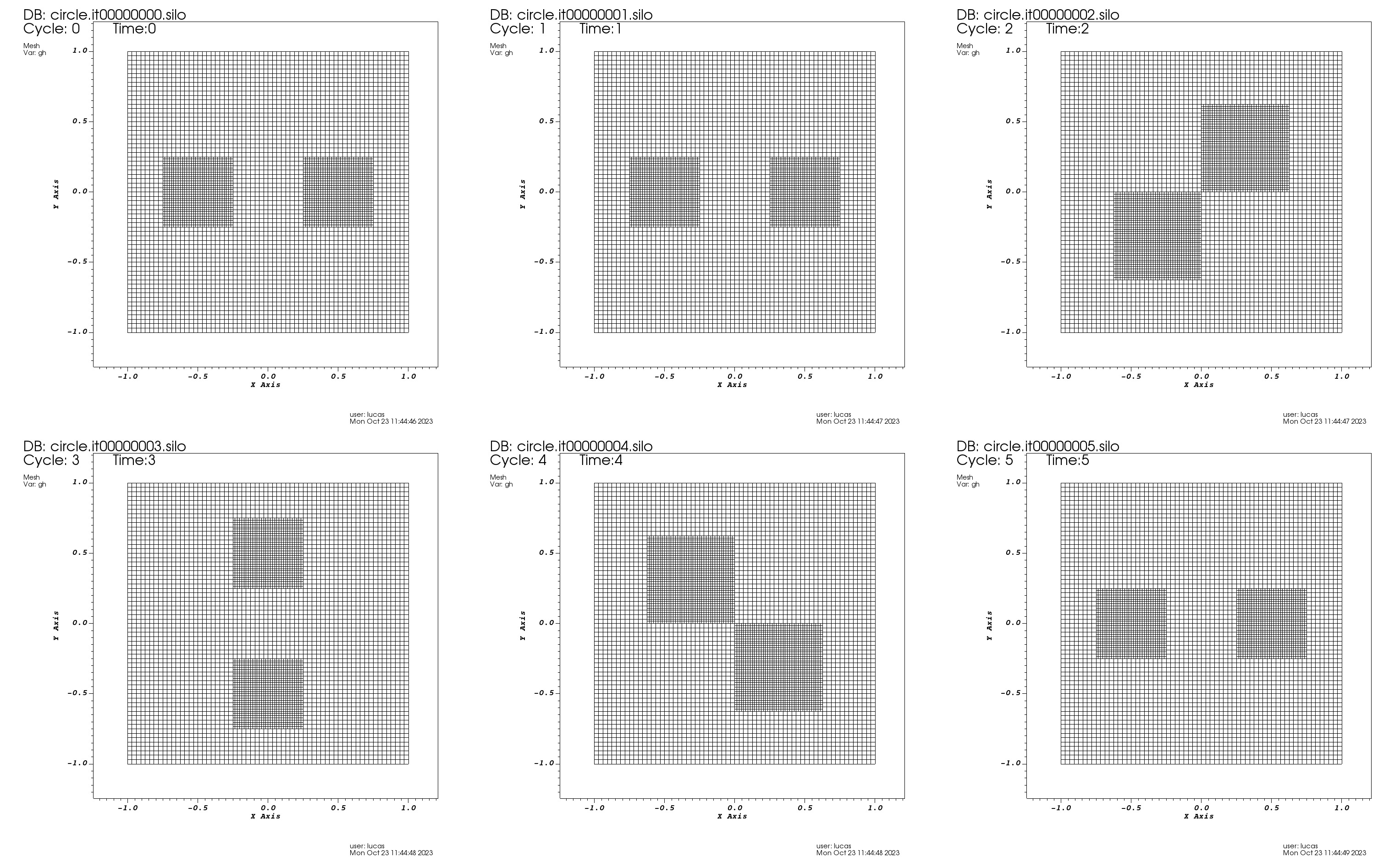
In lines 10 and 13, we read BoxInBox parameters for the initial positions of the boxes. In line 16-21 those positions are updated in a way that the boxes centers describe a circle around the origin. At each time, the boxes move \(\pi /4\) radians around the origin in a counterclockwise fashion. Figure 1 shows 6 still frames of the boxes motions around the origin. All panels are \(z=0\) slices of the grid hierarchy and time and iteration values are provided for each panel. These plots were produced with the VisIt visualization software with CarpetX producing silo data files as output (see Sec. 12 for more details on how to visualize and post-process CarpetX data). The data can be reproduced by running the circle.par parameter file, provided in the par folder of the MovingBoxToy thorn. An animated version of Fig. 1 can be found in the doc folder of the CarpetX thorn under the name animated_boxes.gif.
CarpetX supports non-fixed (adaptive) mesh refinement. For cell level control of AMR, CarpetXRegridError provides users with a cell centered and non-checkpointed grid function called regrid_error. Users are responsible for filling this grid function with real value however they see fit. Once it is filled, the configuration parameter CarpetX::regrid_error_threshold controls regridding: If the values stored in regrid_error are larger than what is set in regrid_error_threshold, the region gets refined. Additionally, the configuration parameter CarpetX::regrid_every controls how many iterations should pass before checking if the error threshold has been exceeded. The parameter CarpetX::max_num_levels controls the maximum number of allowed refinement levels.
Note that CarpetX does not provide a “standardized” regrid error routine. This is because refinement criteria are highly specific to the problem being solved via AMR, and thus there is no one size fits all error criteria. This might seem inconvenient, but ultimately it allows for users to have higher degrees of customization in their AMR codes. For demonstration purposes, we shall now provide a routine that estimates the regrinding error as TODO: what? Provide a good starter example. This implementation could be used as a starting point for codes that wish to use different error criteria in their AMR grids.
1  extern "C" void EstimateError(CCTK_ARGUMENTS) {
2  DECLARE_CCTK_ARGUMENTSX_EstimateError;
3  DECLARE_CCTK_PARAMETERS;
4
5  // The template indices indicate this a loop over cell centers
6  // Remember that regrid_error is a cell centered grid function
7  grid.loop_int_device<1, 1, 1>(
8      grid.nghostzones,
9      [=] (const Loop::PointDesc &p) {
10        // TODO: Give a simple example
11        regrid_error(p.I) = 0.0;
12      });
13}
Once defined, EstimateError should be scheduled in both the postinitial and poststep bins. The poststep bin gets called right after a new state vector has been calculated, and is thus the proper place to analyze it. The postinitial scheduling is also necessary for computing the initial refinement after initial conditions have been set up. A thorn making use of the regrid_error AMR mechanism should then add the following to its schedule.ccl file:
1  SCHEDULE EstimateError AT postinitial
2  {
3    LANG: C
4    READS: state(everywhere)
5    WRITES: CarpetXRegrid::regrid_error(interior)
6  } "Estimate error for regridding"
7
8  SCHEDULE EstimateError AT poststep
9  {
10    LANG: C
11    READS: state(everywhere)
12    WRITES: CarpetXRegrid::regrid_error(interior)
13  } "Estimate error for regridding"
Prolongation refers to the interpolation of data on coarse grid into a finer grid. CarpetX allows users to control how this propagation of data will be executed via the parameter CarpetX::prolongation_type, whose possible values are detailed in Tab. 7. Additionally, other aspects of the prolongation operator can be controlled with the parameters detailed in Tab. 8
| Method | Description |
| "interpolate" | Interpolate between data points |
| "conservative" | Interpolate cell averages, ensuring conservation |
| "ddf" | Interpolate in vertex centered and conserve in cell centered directions |
| "ddf-eno" | Interpolate in vertex centered and ENO-conserve in cell centered directions |
| "ddf-hermite" | Hermite-interpolate in vertex centered and conserve in cell centered directions |
| "natural" | Interpolate in vertex centered and conserve in cell centered directions, using the same order |
| "poly-cons3lfb" | Interpolate polynomially in vertex centered directions and conserve with 3rd order accuracy and a linear fallback in cell centered directions |
| Parameter | Type | Default value | Description |
| prolongation_order | Integer larger than 0 | 1 | Controls the order of the interpolation in prolongation |
| do_restrict | Boolean | yes | Automatically restrict fine to coarse grid functions |
| restrict_during_sync | Boolean | yes | Restrict fine to coarse grid functions when syncing |
CarpetX provides a way of setting up standard boundary conditions and symmetry conditions (to be applied on grid boundaries) via parameter files and grid function tags. More complex boundary conditions can be implemented by users but doing so is not often an easy task due to how AMReX works internally.
The following boundary condition types can be specified:
"none": Don’t apply any boundary condition to the grid. This is the default setting for all boundaries.
"dirichlet": Dirichlet boundary conditions.
"linear extrapolation": Linearly extrapolate interior values to boundary values.
"neumann": Neumann boundary conditions.
"robin": Robin boundary conditions.
Remember that, given a function \(f(x,y,z)\) that satisfies a given PDE in a domain \(\Omega \subset \mathbb {R}^n\) whose boundary is denoted by \(\partial \Omega \), a Dirichlet boundary condition imposes that \begin {equation} f(x,y,z) = g \quad \forall (x,y,z) \in \partial \Omega , \label {eq:dirichlet} \end {equation} a Neumann boundary condition imposes that \begin {equation} \frac {\partial f}{\partial \mathbf {n}} = g \quad \forall (x,y,z) \in \partial \Omega , \label {eq:neumann} \end {equation} where \(\mathbf {n}\) is the normal to the boundary \(\partial \Omega \) and a Robin boundary condition imposes that \begin {equation} a f + b \frac {\partial f}{\partial \mathbf {n}} = g \quad \forall (x,y,z) \in \partial \Omega . \label {eq:robin} \end {equation}
The type of boundary condition in all 6 grid faces can be configured independently via the parameters described in Tab. 9.
| Parameter | Description |
| boundary_x | Boundary condition at lower \(x\) boundary |
| boundary_upper_x | Boundary condition at upper \(x\) boundary |
| boundary_y | Boundary condition at lower \(y\) boundary |
| boundary_upper_y | Boundary condition at upper \(y\) boundary |
| boundary_z | Boundary condition at lower \(z\) boundary |
| boundary_upper_z | Boundary condition at upper \(z\) boundary |
Once boundary types are chosen, they are applied to all grid functions. Users may override the global configuration for a specific set of grid function in which different boundary conditions should be applied to. This is done by passing a list of space (or new line) separated strings to the appropriate parameter, depending on which boundary condition(s) should be overridden. These parameters are of the form
CarpetX::<boundary condition name>_<direction>_vars = "..."
where <boundary condition name> is one of
dirichlet
linear_extrapolation
neumann
robin
and <direction> is one of
x
y
z
upper_x
upper_y
upper_z
In order to set the actual values of Dirichlet, Neumann and Robin boundary conditions, users can specify values via the TAGS mechanism in interface.ccl, detailed in Sec. 3.3. Note that it is only possible to set the quantity \(g\) in Eqs (4)-(6). The syntax is as follows
1  # For Dirichlet BCs
2  CCTK_<type> <group-name> TAGS=’dirichlet_values={1.0}’
3  {
4    ...
5  } "A group of variables"
6
7  # For Neumman BCs
8  CCTK_<type> <group-name> TAGS=’neumann_values={1.0}’
9  {
10    ...
11  } "A group of variables"
12
13  # For Robin BCs
14  CCTK_<type> <group-name> TAGS=’robin_values={1.0}’
15  {
16    ...
17  } "A group of variables"
If a variable group contains multiple variables or multiple boundary conditions, simply append the boundary values to the brace enclose list of boundary values and add another boundary condition as a tag. For example, consider the 3-metric variable group declared in the ADMBaseX thorn bundled with CarpetX, which consists of 6 grid functions each with their own Dirichlet and Robin boundary condition values:
1  CCTK_REAL metric TYPE=gf TAGS=’dirichlet_values={1.0 0.0 0.0   1.0 0.0   1.0} robin_values={1.0 0.0 0.0   1.0 0.0   1.0} ...’
2  {
3    gxx gxy gxz gyy gyz gzz
4  } "ADM 3-metric g_ij"
CarpetX supports two types of symmetry boundary conditions: Reflections and periodicity. Each of these conditions can be set individually for each grid face as with boundary conditions. To Set reflective symmetry conditions, the parameters in Tab. 10 are available. To set periodicity, the parameters in Tab. 11 are provided.
| Parameter | Description |
| reflection_x | Reflection symmetry at lower \(x\) boundary |
| reflection_upper_x | Reflection symmetry at upper \(x\) boundary |
| reflection_y | Reflection symmetry at lower \(y\) boundary |
| reflection_upper_y | Reflection symmetry at upper \(y\) boundary |
| reflection_z | Reflection symmetry at lower \(z\) boundary |
| reflection_upper_z | Reflection symmetry at upper \(z\) boundary |
| Parameter | Description |
| periodic_x | Periodic \(x\) boundary |
| periodic_x | periodic \(y\) boundary |
| periodic_y | Periodic \(z\) boundary |
The recommended way of applying custom boundary conditions is to write them to the RHS of the evolution system. Let us once again consider the function that computes the RHS of Eqs. (??)-(??) presented in Sec. 5 modified to compute boundary conditions:
1extern "C" void LoopExample_RHS(CCTK_ARGUMENTS) {
2  DECLARE_CCTK_ARGUMENTS_LoopExample_RHS;
3  DECLARE_CCTK_PARAMETERS;
4
5  // The grid variable is implicitly defined via the CCTK macros
6  // A 0/1 in template parameters indicate that a grid is vertex/cell centered
7  grid.loop_int<0, 0, 0>(
8    grid.nghostzones,
9
10    // The loop lambda
11    [=] (const Loop::PointDesc &p) {
12      using std::pow;
13
14      // Instead of computing values for each direction expression
15      // explicitly we will use a loop to save us from some typing
16      // ddu will store the partial results for each direction
17      Arith::vect<CCTK_REAL, dim> ddu;
18
19      // Loop over directions
20      for (int d = 0; d < dim; ++d) {
21
22        // Boundary associated with xmin ymin and zmin
23        if (p.BI[d] < 0) {
24          ddu[d] = 0;
25        }
26        // Boundary associated with xmax ymax and zmax
27        else if (p.BI[d] > 0) {
28          ddu[d] = 0;
29        }
30        // interior
31        else {
32          ddu[d] = (u(p.I - p.DI[d]) - 2 * u(p.I) + u(p.I + p.DI[d])) /
33                    pow(p.DX[d], 2);
34        }
35      }
36
37      u_rhs(p.I) = rho(p.I);
38      rho_rhs(p.I) = ddu[0] + ddu[1] + ddu[2];
39
40    } // Ending of the loop lambda
41  ); // Ending of the loop_int call
42}
Instead of computing derivatives and boundaries for each direction explicitly, we use a loop over each direction, written on line 20. The if branches on lines 23-25 and 27-29 set the values of the RHS of the system in the boundaries associated with the xyz_min values and xyz_max values, respectively. In these case, we are setting boundary values to \(0\), but users would use whatever boundary condition they require. The takeaway message of this example is to note how one can access boundary points, instead of what to write to those points.
The recommended way of performing interpolation is using the flesh interface for interpolation by calling CCTK_InterpGridArrays(), as documented on Sec. C1.7.4 of the Cactus user guide and with detailed API description in Sec. A149 of the Cactus reference manual.
Internally, this functionality is implemented by the DriverInterpolate function. If users desire, they can call it directly instead of using CCTK_InterpGridArrays(). In order to do so, users must add the following to their interface.ccl file
1  CCTK_INT FUNCTION DriverInterpolate(
2    CCTK_POINTER_TO_CONST IN cctkGH,
3    CCTK_INT IN N_dims,
4    CCTK_INT IN local_interp_handle,
5    CCTK_INT IN param_table_handle,
6    CCTK_INT IN coord_system_handle,
7    CCTK_INT IN N_interp_points,
8    CCTK_INT IN interp_coords_type,
9    CCTK_POINTER_TO_CONST ARRAY IN interp_coords,
10    CCTK_INT IN N_input_arrays,
11    CCTK_INT ARRAY IN input_array_indices,
12    CCTK_INT IN N_output_arrays,
13    CCTK_INT ARRAY IN output_array_types,
14    CCTK_POINTER ARRAY IN output_arrays)
15  REQUIRES FUNCTION DriverInterpolate
Note that DriverInterpolate and CCTK_InterpGridArrays() receive exactly the same arguments (again, a complete description of these is given in Sec. A149 of the Cactus reference manual) but some arguments are unused by CarpetX. These are coord_system_handle, interp_coords_type_code, output_array_type_codes and interp_handle. Here’s and example of a DriverInterpolate call where these ignored parameters are set to zero:
1  // DriverInterpolate arguments that aren’t currently used
2  CCTK_INT const coord_system_handle = 0;
3  CCTK_INT const interp_coords_type_code = 0;
4  CCTK_INT const output_array_type_codes[1] = {0};
5  int interp_handle = 0;
6
7  // We assume that the other (non-ignored) parameters exist
8  // within the scope but are ommited from this snippet for clarity
9  DriverInterpolate(
10      cctkGH, N_dims, interp_handle, param_table_handle, coord_system_handle,
11      npoints, interp_coords_type_code, interp_coords, nvars, (int const*const)varinds,
12      nvars, output_array_type_codes, output_array);
Lastly, to control the order of the interpolation operators, users can set the CarpetX::interpolation_order parameter, which defaults to 1 and must be greater than 0.
When running on CPUs, AMReX will divide the grid in boxes whose sizes are controlled by blocking_factor and max_grid_size parameter families. These will be distributed over MPI ranks and each rank will subdivide the boxes on tiles. This subdivision into tiles is only logical (not in memory). Threads may then process tiles in any random order. When running on GPU’s, tiling is disabled and AMReX tries to assign one GPU per MPI process. If there are more MPI processes than grids to distribute, some MPI process may become idle. To prevent this from happening, the CarpetX::refine_grid_layout (see bellow) can be used to ensure that each MPI rank processes at least one grid.
CarpetX allows users to control AMReX’s underlying load balancing mechanism by exposing AMReX parameters to Cactus parameter files. We shall now describe these parameters and their functionality.
AMReX will divide the domain in every direction so that each grid is no longer than max_grid_size in that direction. It defaults to 32 in each coordinate direction.
Constrain grid creation so that each grid must be divisible by blocking_factor. This implies that both the domain (at each level) and max_grid_size must be divisible by blocking_factor, and that blocking_factor must be either 1 or a power of 2. It defaults to 8 in every direction.
If set to "yes" and the number of grids created is less than the number of processors (\(N_\text {grids} < N_\text {procs}\)), then grids will be further subdivided until \(N_\text {grids} \geq N_\text {procs}\). If subdividing the grids to achieve \(N_\text {grids} \geq N_\text {procs}\) would violate the blocking_factor criterion then additional grids are not created and the number of grids will remain less than the number of processors. It defaults to "yes"
Because mesh refinement in AMReXis done per-cell (see sec. 7.2 for further details), a refinement region may be irregular. AMReX can only deal with logically cubical grids, thus a refinement region will be replaced by a new grid consisting of coarse and finer boxes on the region. Due to this “discretization” of the refinement region, more cells will be refined than necessary. Refining too many points becomes obviously inefficient. Conversely, refining too few points is also non-ideal, as it leads to a grid structure consisting of many small boxes. “Grid efficiency” then refers to the ratio of the points that need to be refined over the points that actually are refined in the new grid structure. This steers AMReX’s eagerness to combine smaller boxes into larger ones by refining more points. The default value for this parameter is \(0.7\)
Controls tile sizes. In order to be cache efficient, tiling is disabled in the x direction because these elements are not stored contiguously in memory. The default values for max_tile_size are given in Tab. 12. These default values were found trough experimentation. Users are encouraged to change them in order to achieve optimal performance in their machines and use cases.
| Parameter | Default value |
| max_tile_size_x | \(1024000\) (disabled) |
| max_tile_size_y | \(16\) |
| max_tile_size_z | \(32\) |
Profiling refers to the act of collecting runtime and other performance data on the execution of an application in order to improve its performance characteristics. The recommended way of profiling CarpetX applications is using HPCToolkit. We recommend that user first read the software’s documentation thoroughly.
Installing HPCToolkit on an HPC system will probably require the help of the system’s administrators. Once installed, the application should be launched with the hpcrun command, which will automatically collect performance data from the launched application. To profile CarpetX while using an HPC system, the recommended steps are:
Launch an interactive section with the cluster’s job system. In this session, the mpirun and hpcrun commands should be available.
Navigate to the directory where the Cactus executable is located. Given a configuration named config-name, the executable is located in Cactus/exe/cactus_config-name.
Select a parameter file to execute and gather performance information on. Let us call it perf.par and suppose that it is located in Cactus/exe/.
Assuming that the system’s MPI launcher is called mpirun, to profile a CPU application, issue
1 mpirun hpcrun ./cactus_config-name perf.par
To profile a GPU application, issue
1 mpirun hpcrun -e gpu=<vendor> ./cactus_config-name perf.par
where <vendor> is either nvidia or amd, depending on which GPU chips are available in the system.
After Cactus completes the evolution, a new folder called hpctoolkit-cactus_config-name-measurements will be created on the same directory where hpcrun was executed. HPCToolkit needs to recover program structure in order to create better profiling information. To do that, issue
1 hpcstruct hpctoolkit-cactus_config-name-measurements
Finally, to have HPCToolkit analyze measurements and attribute it to source code, issue
1 hpcprof hpctoolkit-cactus_config-name-measurements
This will generate the hpctoolkit-cactus_config-name-database folder, which can be used with HPCToolkit’s provided profile visualization tool called hpcviewer. See chapter 10 of the HPCToolkit manual for usage details.
CarpetX outputs data in the following formats: Silo, openPMD (with various backends), Adios2 and TSV. For each output format, users can choose what and how frequently variables will be written to disk. In the following sections we will provide details to each format.
The TSV acronym stands for Tab Separated Values. This is a plain text format in which data is written to files in rows (lines) and columns, each column separated by a tab character. These formats are very easy to hand parse and manipulate or post-process. Many open source tools are also available for reading this format out of the box (see for instance the Python framework Pandas). There are however two important disadvantages in using plain text formats: The first is a loss of precision when converting floating point numbers from binary to string representation and converting from string back into binary form, due to the way floating point numbers work. The second is compactness. While a 16 digit double precision floating point number takes 8 bytes to be represented in binary form, it requires at least 17 bytes (1 byte per digit plus the floating point dot) to be represented as a string. For these reasons, this format is not recommended to production runs or to complex data analysis. It is useful however, for quick and easy visualizations or diagnostics of data. It is also useful when other, more sophisticated formats are not available.
To control TSV output, CarpetX provides the parameters described in Tab. 12.1
| Parameter | Type | Default Value | Description |
| out_tsv | Boolean | "yes" | Whether to produce TSV output |
| out_tsv_vars | String | Empty string | Space or newline separated string of grid functions to output |
| out_tsv_every | Integer | \(-1\) | If set to \(-1\), output is produced as often as the setting of IO::out_every. If set to \(0\), output is never produced. If set to \(1\) or larger, output every that many iterations |
As an example, to output the grid functions of WaveToyX as TSV files every 2 iterations, one would write in their parameter file the following excerpt
1  CarpetX::out_tsv = yes
2  CarpetX::out_tsv_every = 2
3  CarpetX::out_tsv_vars = "
4    WaveToyX::state
5    WaveToyX::rhs
6    WaveToyX::energy
7    WaveToyX::error
8"
The Silo format (see here for more information) is the native file format of the VisIt data visualization tool. Given its native support in VisIt, silo files are good for direct visualization of simulation data and grids (Fig. 1 of this document as well as the animated_boxes.gif file in the documentation folder were both created with VisIt).
To control SILO output, CarpetX provides the parameters described in Tab. 12.2
| Parameter | Type | Default Value | Description |
| out_silo_vars | String | Empty string | Space or newline separated string of grid functions to output |
| out_silo_every | Integer | \(-1\) | If set to \(-1\), output is produced as often as the setting of IO::out_every. If set to \(0\), output is never produced. If set to \(1\) or larger, output every that many iterations |
As an example, to output the grid functions of WaveToyX as SILO files every 2 iterations, one would write in their parameter file the following excerpt
1  CarpetX::out_silo_every = 2
2  CarpetX::out_silo_vars = "
3    WaveToyX::state
4    WaveToyX::rhs
5    WaveToyX::energy
6    WaveToyX::error
7"
openPMD stands for “open standard for particle-mesh data files”. Strictly speaking, it is not a file format, but a standard for meta-data, naming schemes and file organization. openPMD is thus “backed” by usual hierarchical binary data formats, such as HDF5 and Adios2, both supported by CarpetX. Put simply, openPMD specifies a standardized and interchangeable way of organizing data within HDF5 and Adios2 files.
To control openPMD output, CarpetX provides the parameters described in Tab. 12.3
| Parameter | Type | Default Value | Description |
| out_openpmd_vars | String | Empty string | Space or newline separated string of grid functions to output |
| out_openpmd_every | Integer | \(-1\) | If set to \(-1\), output is produced as often as the setting of IO::out_every. If set to \(0\), output is never produced. If set to \(1\) or larger, output every that many iterations |
Additionally, it is possible to control which “backing” format to use with openPMD via the CarpetX::openpmd_format parameter, whose possible string values are listed in Tab 12.3
| Value | Description |
| "HDF5" | The Hierarchical Data Format, version 5 (see here) |
| "ADIOS1" | The Adaptable I/O System version 1 (see here) |
| "ADIOS2" | The Adaptable I/O System version 2 (see here). Requires openPMD_api \(< 0.15\) |
| "ADIOS2_BP" | ADIOS2 native binary-pack. Requires openPMD_api \(\geq 0.15\) |
| "ADIOS2_BP4" | ADIOS2 native binary-pack version 4 (see here). Requires openPMD_api \(\geq 0.15\) |
| "ADIOS2_BP5" | ADIOS2 native binary-pack version 5 (see here). Requires openPMD_api \(\geq 0.15\) |
| "ADIOS2_SST" | ADIOS2 Sustainable Staging Transport (see hee) |
| "ADIOS2_SSC" | ADIOS2 Strong Staging Coupler (see here) |
| "JSON" | JavaScript Object Notation (see here) |
When using openPMD output, CarpetX can produce files that can be visualized with VisIt. To do that for WaveToyX, for example, the following excerpt would be added to a parameter file
1  # It is very important to produce BP4 files, as BP5
2  # cannot be imported into VisIt at the time of writing
3  CarpetX::openpmd_format = "ADIOS2_BP4"
4
5  CarpetX::out_openpmd_vars = "
6      WaveToyX::state
7      WaveToyX::rhs
8      WaveToyX::energy
9      WaveToyX::error
10  "
When loading data into VisIt, users must open the *.pmd.visit file produced together with the simulation output. It is also imperative to select the file format as ADIOS2 in VisIt’s file selector window, otherwise the files will not be loaded correctly.
In addition to VisIt, users can find in the CarpetX/doc/openpmd-plot folder a sample Python script for extracting and plotting data from CarpetX produced openPMD files. The best way to interact with the script is using a Python virtual environment. First, navigate to the CarpetX/doc/openpmd-plot and issue the following commands:
1python -m venv venv             # Creates the virtual environment.
2source venv/bin/activate        # Activates the virtual environment.
3pip install -r requirements.txy # Installs required packages.
4python plot-zslice.py -h        # See the options available.
5deactivate                      # Exits the environment when done.
To output pure ADIOS2 BP5 files, (without openPMD formatting), users can use the parameters described in Tab. 12.4. Note that this output mode produces BP5 files, which cannot be read by VisIt (at the time of writing). Users may have to rely on their own tools and scripts for data processing and visualization.
| Parameter | Type | Default Value | Description |
| out_adios2_vars | String | Empty string | Space or newline separated string of grid functions to output |
| out_adios2_every | Integer | \(-1\) | If set to \(-1\), output is produced as often as the setting of IO::out_every. If set to \(0\), output is never produced. If set to \(1\) or larger, output every that many iterations |
As an example, to produce ADIOS2 files at every \(2\) time steps in WaveToyX, users would use the following excerpt
1  CarpetX::out_adios2_every = 2
2  CarpetX::out_adios2_vars = "
3    WaveToyX::state
4    WaveToyX::rhs
5    WaveToyX::energy
6    WaveToyX::error
7"
CarpetXcan output various norms of grid functions, such as min., max., L2 and others. This output works similarly to the previously described methods. To control norm output, the parameters in Tab. 12.5 are provided.
| Parameter | Type | Default Value | Description |
| out_norm_vars | String | Empty string | Space or newline separated string of grid functions to output |
| out_norm_every | Integer | \(-1\) | If set to \(-1\), output is produced as often as the setting of IO::out_every. If set to \(0\), output is never produced. If set to \(1\) or larger, output every that many iterations |
For example, to output openPMD and norms for the WaveToyX thorn grid functions, the following excerpt could be added to a parameter file
1  CarpetX::out_norm_every = 2
2
3  # Here we choose to output only norms of the error grid function
4  CarpetX::out_norm_vars = "
5      WaveToyX::error
6  "
7
8  # It is very important to produce BP4 files, as BP5
9  # cannot be imported into VisIt at the time of writing
10  CarpetX::openpmd_format = "ADIOS2_BP4"
11
12  CarpetX::out_openpmd_vars = "
13      WaveToyX::state
14      WaveToyX::rhs
15      WaveToyX::energy
16      WaveToyX::error
17  "
CarpetX can produce a file called performance.yaml with various performance timers for certain iterations of a simulation. This output mirrors that of stdout and may be useful for thorn developers while benchmarking their codes. Controlling performance output is done similarly as to other types of output. The parameters for controlling it are detailed in Tab 12.6
| Parameter | Type | Default Value | Description |
| out_performance | Boolean | "yes" | Whether to produce performance data in YAML format. |
| out_performance_every | Integer | \(-1\) | If set to \(-1\), output is produced as often as the setting of IO::out_every. If set to \(0\), output is never produced. If set to \(1\) or larger, output every that many iterations. |
As an example, to have performance measurements output for a simulation every 2 iterations, the following parameters may be added to a parameter file
1  CarpetX::out_performance = yes
2  CarpetX::out_performance_every = 2
To debug CarpetX applications, users have access to the following parameters:
verbose: A boolean parameter that controls weather or not CarpetX produces verbose output. This output details more of what the driver is doing internally, aiding users in finding bugs. Its default value is no.
poison_undefined_values: Sets undefined grid point values to NaN (not a number). By visualizing locations where grid functions contain NaNs, users can determine which grid points are not being filled correctly. Its default value is yes.
| amrex_parameters | Scope: private | STRING |
| Description: Additional AMReX parameters
| ||
| Range | Default: (none) | |
| do nothing
| ||
| [  ]+=.* ]+=.* | keyword=value
| |
| blocking_factor_x | Scope: private | INT |
| Description: Blocking factor
| ||
| Range | Default: 8 | |
| 1:* | ||
| blocking_factor_y | Scope: private | INT |
| Description: Blocking factor
| ||
| Range | Default: 8 | |
| 1:* | ||
| blocking_factor_z | Scope: private | INT |
| Description: Blocking factor
| ||
| Range | Default: 8 | |
| 1:* | must be a power of 2
| |
| boundary_upper_x | Scope: private | KEYWORD |
| Description: Boundary condition at upper x boundary
| ||
| Range | Default: none | |
| none | don’t apply any boundary
| |
| dirichlet | Dirichlet
| |
| linear extrapolation | Linear extrapolation
| |
| neumann | Neumann
| |
| robin | Robin
| |
| boundary_upper_y | Scope: private | KEYWORD |
| Description: Boundary condition at upper y boundary
| ||
| Range | Default: none | |
| none | don’t apply any boundary
| |
| dirichlet | Dirichlet
| |
| linear extrapolation | Linear extrapolation
| |
| neumann | Neumann
| |
| robin | Robin
| |
| boundary_upper_z | Scope: private | KEYWORD |
| Description: Boundary condition at upper z boundary
| ||
| Range | Default: none | |
| none | don’t apply any boundary
| |
| dirichlet | Dirichlet
| |
| linear extrapolation | Linear extrapolation
| |
| neumann | Neumann
| |
| robin | Robin
| |
| boundary_x | Scope: private | KEYWORD |
| Description: Boundary condition at lower x boundary
| ||
| Range | Default: none | |
| none | don’t apply any boundary
| |
| dirichlet | Dirichlet
| |
| linear extrapolation | Linear extrapolation
| |
| neumann | Neumann
| |
| robin | Robin
| |
| boundary_y | Scope: private | KEYWORD |
| Description: Boundary condition at lower y boundary
| ||
| Range | Default: none | |
| none | don’t apply any boundary
| |
| dirichlet | Dirichlet
| |
| linear extrapolation | Linear extrapolation
| |
| neumann | Neumann
| |
| robin | Robin
| |
| boundary_z | Scope: private | KEYWORD |
| Description: Boundary condition at lower z boundary
| ||
| Range | Default: none | |
| none | don’t apply any boundary
| |
| dirichlet | Dirichlet
| |
| linear extrapolation | Linear extrapolation
| |
| neumann | Neumann
| |
| robin | Robin
| |
| checkpoint_method | Scope: private | KEYWORD |
| Description: I/O method for checkpointing
| ||
| Range | Default: error | |
| error | Abort with error instead of checkpointing
| |
| openpmd | ||
| silo | ||
| dirichlet_upper_x_vars | Scope: private | STRING |
| Description: Override boundary condition at upper x boundary
| ||
| Range | Default: (none) | |
| .* | ||
| dirichlet_upper_y_vars | Scope: private | STRING |
| Description: Override boundary condition at upper y boundary
| ||
| Range | Default: (none) | |
| .* | ||
| dirichlet_upper_z_vars | Scope: private | STRING |
| Description: Override boundary condition at upper z boundary
| ||
| Range | Default: (none) | |
| .* | ||
| dirichlet_x_vars | Scope: private | STRING |
| Description: Override boundary condition at lower x boundary
| ||
| Range | Default: (none) | |
| .* | ||
| dirichlet_y_vars | Scope: private | STRING |
| Description: Override boundary condition at lower y boundary
| ||
| Range | Default: (none) | |
| .* | ||
| dirichlet_z_vars | Scope: private | STRING |
| Description: Override boundary condition at lower z boundary
| ||
| Range | Default: (none) | |
| .* | ||
| do_reflux | Scope: private | BOOLEAN |
| Description: Manage flux registers to ensure conservation
| ||
| Default: yes | ||
| do_restrict | Scope: private | BOOLEAN |
| Description: Automatically restrict fine to coarse grid functions
| ||
| Default: yes | ||
| dtfac | Scope: private | REAL |
| Description: The standard timestep condition dt = dtfac*min(delta_space)
| ||
| Range | Default: 0.5 | |
| *:* | ||
| filereader_method | Scope: private | KEYWORD |
| Description: I/O method for file reader
| ||
| Range | Default: error | |
| error | Abort with error when file reader is used
| |
| openpmd | ||
| silo | ||
| ghost_size | Scope: private | INT |
| Description: Number of ghost zones
| ||
| Range | Default: -1 | |
| -1 | use ghost_size_[xyz]
| |
| 0:* | ||
| ghost_size_x | Scope: private | INT |
| Description: Number of ghost zones
| ||
| Range | Default: 1 | |
| 0:* | ||
| ghost_size_y | Scope: private | INT |
| Description: Number of ghost zones
| ||
| Range | Default: 1 | |
| 0:* | ||
| ghost_size_z | Scope: private | INT |
| Description: Number of ghost zones
| ||
| Range | Default: 1 | |
| 0:* | ||
| gpu_sync_after_every_kernel | Scope: private | BOOLEAN |
| Description: Call amrex::Gpu::streamSynchronize after every kernel (EXPENSIVE)
| ||
| Default: no | ||
| grid_efficiency | Scope: private | REAL |
| Description: Minimum AMR grid efficiency
| ||
| Range | Default: 0.7 | |
| 0.0:* | ||
| interpolation_order | Scope: private | INT |
| Description: Interpolation order
| ||
| Range | Default: 1 | |
| 0:* | ||
| kernel_launch_method | Scope: private | KEYWORD |
| Description: Kernel launch method
| ||
| Range | Default: default | |
| serial | no parallelism
| |
| openmp | use OpenMP
| |
| cuda | target CUDA
| |
| default
| Use OpenMP for CPU builds and CUDA for GPU
builds
| |
| linear_extrapolation_upper_x_vars | Scope: private | STRING |
| Description: Override boundary condition at upper x boundary
| ||
| Range | Default: (none) | |
| .* | ||
| linear_extrapolation_upper_y_vars | Scope: private | STRING |
| Description: Override boundary condition at upper y boundary
| ||
| Range | Default: (none) | |
| .* | ||
| linear_extrapolation_upper_z_vars | Scope: private | STRING |
| Description: Override boundary condition at upper z boundary
| ||
| Range | Default: (none) | |
| .* | ||
| linear_extrapolation_x_vars | Scope: private | STRING |
| Description: Override boundary condition at lower x boundary
| ||
| Range | Default: (none) | |
| .* | ||
| linear_extrapolation_y_vars | Scope: private | STRING |
| Description: Override boundary condition at lower y boundary
| ||
| Range | Default: (none) | |
| .* | ||
| linear_extrapolation_z_vars | Scope: private | STRING |
| Description: Override boundary condition at lower z boundary
| ||
| Range | Default: (none) | |
| .* | ||
| max_grid_size_x | Scope: private | INT |
| Description: Maximum grid size
| ||
| Range | Default: 32 | |
| 1:* | must be a multiple of the blocking factor
| |
| max_grid_size_y | Scope: private | INT |
| Description: Maximum grid size
| ||
| Range | Default: 32 | |
| 1:* | must be a multiple of the blocking factor
| |
| max_grid_size_z | Scope: private | INT |
| Description: Maximum grid size
| ||
| Range | Default: 32 | |
| 1:* | must be a multiple of the blocking factor
| |
| max_grid_sizes_x | Scope: private | INT |
| Description: Maximum grid size
| ||
| Range | Default: -1 | |
| -1 | use value from max_grid_size_x
| |
| 1:* | must be a multiple of the blocking factor
| |
| max_grid_sizes_y | Scope: private | INT |
| Description: Maximum grid size
| ||
| Range | Default: -1 | |
| -1 | use value from max_grid_size_y
| |
| 1:* | must be a multiple of the blocking factor
| |
| max_grid_sizes_z | Scope: private | INT |
| Description: Maximum grid size
| ||
| Range | Default: -1 | |
| -1 | use value from max_grid_size_z
| |
| 1:* | must be a multiple of the blocking factor
| |
| max_num_levels | Scope: private | INT |
| Description: Maximum number of refinement levels
| ||
| Range | Default: 1 | |
| 1:* | ||
| max_tile_size_x | Scope: private | INT |
| Description: Maximum tile size
| ||
| Range | Default: 1024000 | |
| 1:* | ||
| max_tile_size_y | Scope: private | INT |
| Description: Maximum tile size
| ||
| Range | Default: 16 | |
| 1:* | ||
| max_tile_size_z | Scope: private | INT |
| Description: Maximum tile size
| ||
| Range | Default: 32 | |
| 1:* | ||
| ncells_x | Scope: private | INT |
| Description: Number of grid cells
| ||
| Range | Default: 128 | |
| 1:* | must be a multiple of the blocking factor
| |
| ncells_y | Scope: private | INT |
| Description: Number of grid cells
| ||
| Range | Default: 128 | |
| 1:* | must be a multiple of the blocking factor
| |
| ncells_z | Scope: private | INT |
| Description: Number of grid cells
| ||
| Range | Default: 128 | |
| 1:* | must be a multiple of the blocking factor
| |
| neumann_upper_x_vars | Scope: private | STRING |
| Description: Override boundary condition at upper x boundary
| ||
| Range | Default: (none) | |
| .* | ||
| neumann_upper_y_vars | Scope: private | STRING |
| Description: Override boundary condition at upper y boundary
| ||
| Range | Default: (none) | |
| .* | ||
| neumann_upper_z_vars | Scope: private | STRING |
| Description: Override boundary condition at upper z boundary
| ||
| Range | Default: (none) | |
| .* | ||
| neumann_x_vars | Scope: private | STRING |
| Description: Override boundary condition at lower x boundary
| ||
| Range | Default: (none) | |
| .* | ||
| neumann_y_vars | Scope: private | STRING |
| Description: Override boundary condition at lower y boundary
| ||
| Range | Default: (none) | |
| .* | ||
| neumann_z_vars | Scope: private | STRING |
| Description: Override boundary condition at lower z boundary
| ||
| Range | Default: (none) | |
| .* | ||
| openpmd_format | Scope: private | KEYWORD |
| Description: openPMD file format
| ||
| Range | Default: ADIOS2_auto | |
| HDF5 | ||
| ADIOS1
| requires openPMD_api <0.16
| |
| ADIOS2_auto
| Choose ADIOS2 format automatically (either
ADIOS2_BP5 or ADIOS2_BP4)
| |
| ADIOS2 | requires openPMD_api <0.15
| |
| ADIOS2_BP | requires openPMD_api >=0.15
| |
| ADIOS2_BP4 | requires openPMD_api >=0.15
| |
| ADIOS2_BP5 | requires openPMD_api >=0.15
| |
| ADIOS2_SST | ||
| ADIOS2_SSC | ||
| JSON | ||
| TOML | requires openPMD_api >=0.16
| |
| GENERIC | requires openPMD_api >=0.16
| |
| out_adios2_every | Scope: private | INT |
| Description: Output in ADIOS2 format every that many iterations
| ||
| Range | Default: -1 | |
| -1 | use value of IO::out_every
| |
| never output ADIOS2
| ||
| 1:* | every that many iterations
| |
| out_adios2_vars | Scope: private | STRING |
| Description: Variables to output in ADIOS2 format
| ||
| Range | Default: (none) | |
| .* | ||
| out_metadata | Scope: private | BOOLEAN |
| Description: Output metadata in YAML format?
| ||
| Default: yes | ||
| out_metadata_every | Scope: private | INT |
| Description: Output metadata every that many iterations
| ||
| Range | Default: -1 | |
| -1 | use value of IO::out_every
| |
| never output metadata
| ||
| 1:* | every that many iterations
| |
| out_norm_every | Scope: private | INT |
| Description: Output norms every that many iterations
| ||
| Range | Default: -1 | |
| -1 | use value of IO::out_every
| |
| never output norms
| ||
| 1:* | every that many iterations
| |
| out_norm_omit_sumloc_for_backward_compatibility | Scope: private | BOOLEAN |
| Description: Omit sumloc norms
| ||
| Default: no | ||
| out_norm_omit_unstable | Scope: private | BOOLEAN |
| Description: Omit unstable norms (e.g. maxloc)
| ||
| Default: no | ||
| out_norm_vars | Scope: private | STRING |
| Description: Variables to output as norms
| ||
| Range | Default: (none) | |
| .* | ||
| out_openpmd_every | Scope: private | INT |
| Description: Output in openPMD format every that many iterations
| ||
| Range | Default: -1 | |
| -1 | use value of IO::out_every
| |
| never output openPMD
| ||
| 1:* | every that many iterations
| |
| out_openpmd_vars | Scope: private | STRING |
| Description: Variables to output in openPMD format
| ||
| Range | Default: (none) | |
| .* | ||
| out_performance | Scope: private | BOOLEAN |
| Description: Output performance data in YAML format?
| ||
| Default: yes | ||
| out_performance_every | Scope: private | INT |
| Description: Output performance data every that many iterations
| ||
| Range | Default: -1 | |
| -1 | use value of IO::out_every
| |
| never output performance data
| ||
| 1:* | every that many iterations
| |
| out_plotfile_every | Scope: private | INT |
| Description: Output in plotfile format every that many iterations
| ||
| Range | Default: -1 | |
| -1 | use value of IO::out_every
| |
| never output plotfile
| ||
| 1:* | every that many iterations
| |
| out_plotfile_groups | Scope: private | STRING |
| Description: Groups to output as AMReX plotfile
| ||
| Range | Default: (none) | |
| .* | ||
| out_silo_every | Scope: private | INT |
| Description: Output in Silo format every that many iterations
| ||
| Range | Default: -1 | |
| -1 | use value of IO::out_every
| |
| never output Silo
| ||
| 1:* | every that many iterations
| |
| out_silo_vars | Scope: private | STRING |
| Description: Variables to output in Silo format
| ||
| Range | Default: (none) | |
| .* | ||
| out_tsv | Scope: private | BOOLEAN |
| Description: 3d Output in TSV (tab-separated values) format?
| ||
| Default: no | ||
| out_tsv_every | Scope: private | INT |
| Description: Output in TSV format every that many iterations
| ||
| Range | Default: -1 | |
| -1 | use value of IO::out_every
| |
| never output TSV
| ||
| 1:* | every that many iterations
| |
| out_tsv_vars | Scope: private | STRING |
| Description: Variables to output in 1d TSV format
| ||
| Range | Default: (none) | |
| .* | ||
| poison_undefined_values | Scope: private | BOOLEAN |
| Description: Set undefined grid point values to nan
| ||
| Default: yes | ||
| prolongate_per_group | Scope: private | BOOLEAN |
| Description: Prolongate all variables in a group together
| ||
| Default: no | ||
| prolongation_order | Scope: private | INT |
| Description: Prolongation order
| ||
| Range | Default: 1 | |
| 0:* | ||
| prolongation_type | Scope: private | KEYWORD |
| Description: Prolongation type
| ||
| Range | Default: natural | |
| interpolate | interpolate between data points
| |
| conservative | interpolate cell averages, ensuring conservation
| |
| ddf
| interpolate in vertex centred and conserve (with one
order lower) in cell centred directions
| |
| eno
| interpolate in vertex centred and minmod-conserve
in cell centred directions
| |
| minmod
| interpolate in vertex centred and ENO-conserve in
cell centred directions
| |
| hermite
| ”Hermite-interpolate in vertex centred and conserve
in cell centred directions”
| |
| natural
| interpolate in vertex centred and conserve in cell
centred directions, using the same order
| |
| poly-cons3lfb
| interpolate polynomially in vertex centred directions
and conserve with 3rd order accuracy and a linear
fallback in cell centred directions
| |
| poly-eno3lfb
| interpolate polynomially in vertex centred directions
and use ENO stencils with 3rd order accuracy and a
linear fallback in cell centred directions
| |
| recover_method | Scope: private | KEYWORD |
| Description: I/O method for recovery
| ||
| Range | Default: error | |
| error | Abort with error instead of recovering
| |
| openpmd | ||
| silo | ||
| refine_grid_layout | Scope: private | BOOLEAN |
| Description: Ensure that each MPI process has at least one grid
| ||
| Default: yes | ||
| reflection_upper_x | Scope: private | BOOLEAN |
| Description: Reflection symmetry at the upper x boundary
| ||
| Default: no | ||
| reflection_upper_y | Scope: private | BOOLEAN |
| Description: Reflection symmetry at the upper y boundary
| ||
| Default: no | ||
| reflection_upper_z | Scope: private | BOOLEAN |
| Description: Reflection symmetry at the upper z boundary
| ||
| Default: no | ||
| reflection_x | Scope: private | BOOLEAN |
| Description: Reflection symmetry at the lower x boundary
| ||
| Default: no | ||
| reflection_y | Scope: private | BOOLEAN |
| Description: Reflection symmetry at the lower y boundary
| ||
| Default: no | ||
| reflection_z | Scope: private | BOOLEAN |
| Description: Reflection symmetry at the lower z boundary
| ||
| Default: no | ||
| regrid_error_threshold | Scope: private | REAL |
| Description: Regridding error threshold
| ||
| Range | Default: 1.0 | |
| 0.0:* | ||
| regrid_every | Scope: private | INT |
| Description: Regridding interval
| ||
| Range | Default: (none) | |
| never
| ||
| 1:* | every that many iterations
| |
| restrict_during_sync | Scope: private | BOOLEAN |
| Description: Restrict fine to coarse grid functions when syncing
| ||
| Default: yes | ||
| robin_upper_x_vars | Scope: private | STRING |
| Description: Override boundary condition at upper x boundary
| ||
| Range | Default: (none) | |
| .* | ||
| robin_upper_y_vars | Scope: private | STRING |
| Description: Override boundary condition at upper y boundary
| ||
| Range | Default: (none) | |
| .* | ||
| robin_upper_z_vars | Scope: private | STRING |
| Description: Override boundary condition at upper z boundary
| ||
| Range | Default: (none) | |
| .* | ||
| robin_x_vars | Scope: private | STRING |
| Description: Override boundary condition at lower x boundary
| ||
| Range | Default: (none) | |
| .* | ||
| robin_y_vars | Scope: private | STRING |
| Description: Override boundary condition at lower y boundary
| ||
| Range | Default: (none) | |
| .* | ||
| robin_z_vars | Scope: private | STRING |
| Description: Override boundary condition at lower z boundary
| ||
| Range | Default: (none) | |
| .* | ||
| use_subcycling_wip | Scope: private | BOOLEAN |
| Description: Use subcycling in time
| ||
| Default: no | ||
| verbose | Scope: private | BOOLEAN |
| Description: Verbose output
| ||
| Default: no | ||
| xmax | Scope: private | REAL |
| Description: Domain size (location of vertices)
| ||
| Range | Default: 1.0 | |
| *:* | ||
| xmin | Scope: private | REAL |
| Description: Domain size (location of vertices)
| ||
| Range | Default: -1.0 | |
| *:* | ||
| ymax | Scope: private | REAL |
| Description: Domain size (location of vertices)
| ||
| Range | Default: 1.0 | |
| *:* | ||
| ymin | Scope: private | REAL |
| Description: Domain size (location of vertices)
| ||
| Range | Default: -1.0 | |
| *:* | ||
| zmax | Scope: private | REAL |
| Description: Domain size (location of vertices)
| ||
| Range | Default: 1.0 | |
| *:* | ||
| zmin | Scope: private | REAL |
| Description: Domain size (location of vertices)
| ||
| Range | Default: -1.0 | |
| *:* | ||
| periodic | Scope: restricted | BOOLEAN |
| Description: Periodic boundary conditions
| ||
| Range | Default: no | |
| yes | must be set for any periodic_x,y,z to be effective
| |
| no | no periodicity
| |
| periodic_x | Scope: restricted | BOOLEAN |
| Description: Periodic boundary conditions in x-direction
| ||
| Range | Default: yes | |
| yes | periodic in x direction, requires periodic=yes as well
| |
| no | not periodic in x direction
| |
| periodic_y | Scope: restricted | BOOLEAN |
| Description: Periodic boundary conditions in y-direction
| ||
| Range | Default: yes | |
| yes | periodic in y direction, requires periodic=yes as well
| |
| no | not periodic in y direction
| |
| periodic_z | Scope: restricted | BOOLEAN |
| Description: Periodic boundary conditions in z-direction
| ||
| Range | Default: yes | |
| yes | periodic in z direction, requires periodic=yes as well
| |
| no | not periodic in z direction
| |
| checkpoint_dir | Scope: shared from IO | STRING |
| checkpoint_every | Scope: shared from IO | INT |
| checkpoint_every_walltime_hours | Scope: shared from IO | REAL |
| checkpoint_file | Scope: shared from IO | STRING |
| checkpoint_id | Scope: shared from IO | BOOLEAN |
| checkpoint_on_terminate | Scope: shared from IO | BOOLEAN |
| filereader_id_dir | Scope: shared from IO | STRING |
| filereader_id_files | Scope: shared from IO | STRING |
| filereader_id_vars | Scope: shared from IO | STRING |
| out_dir | Scope: shared from IO | STRING |
| out_every | Scope: shared from IO | INT |
| out_mode | Scope: shared from IO | KEYWORD |
| out_proc_every | Scope: shared from IO | INT |
| out_xline_y | Scope: shared from IO | REAL |
| out_xline_z | Scope: shared from IO | REAL |
| out_yline_x | Scope: shared from IO | REAL |
| out_yline_z | Scope: shared from IO | REAL |
| out_zline_x | Scope: shared from IO | REAL |
| out_zline_y | Scope: shared from IO | REAL |
| recover | Scope: shared from IO | KEYWORD |
| recover_dir | Scope: shared from IO | STRING |
| recover_file | Scope: shared from IO | STRING |
Implements:
driver
Adds header:
driver.hxx
reduction.hxx
Uses header:
silo.hxx
defs.hxx
div.hxx
rational.hxx
simd.hxx
tuple.hxx
vect.hxx
loop.hxx
loop_device.hxx
Provides:
MultiPatch_GetDomainSpecification to
MultiPatch_GetBoundarySizesAndTypes to
GetCallFunctionCount to
GetLoopBoxAll to
GetLoopBoxInt to
CallScheduleGroup to
SolvePoisson to
Interpolate to
DriverInterpolate to
This section lists all the variables which are assigned storage by thorn CarpetX/CarpetX. Storage can either last for the duration of the run (Always means that if this thorn is activated storage will be assigned, Conditional means that if this thorn is activated storage will be assigned for the duration of the run if some condition is met), or can be turned on for the duration of a schedule function.
NONE
CCTK_STARTUP
carpetx_startup
start up the driver
| Language: | c | |
| Type: | function | |
CCTK_RECOVER_PARAMETERS (conditional)
carpetx_recoverparameters
recover parameters
| Language: | c | |
| Options: | meta | |
| Type: | function | |
CCTK_CPINITIAL
carpetx_checkpointinitial
checkpoint initial conditions
| Language: | c | |
| Options: | meta | |
| Type: | function | |
CCTK_CHECKPOINT
carpetx_checkpoint
checkpoint
| Language: | c | |
| Options: | meta | |
| Type: | function | |
CCTK_TERMINATE
carpetx_checkpointterminate
checkpoint before terminating
| Language: | c | |
| Options: | meta | |
| Type: | function | |
CCTK_SHUTDOWN
carpetx_shutdown
shut down the driver
| Language: | c | |
| Options: | meta | |
| Type: | function | |
| Alias Name: | Function Name: |
| CarpetX_Shutdown | Driver_Shutdown |
| CarpetX_Startup | Driver_Startup |